Introduction to gtsummary package

“The {gtsummary} package provides an elegant and flexible way to create publication-ready analytical and summary tables using the R programming language.” https://www.danieldsjoberg.com/gtsummary/

Introduction

I ran across this amazing package on the datascience side of Twitter. The magic is the combination of creating publication ready output, but being immensely flexible with other parts of R.

Goals

In this real world example, we will use gtsummary to perform both statistics and visuals (tables) for a publication in process.

1. Create a summary demographics table (Part 1)
2. Compare response variables between groups (Part 2)

The dataset consists of several event-related potential (ERP) responses collected from electroencephalography (EEG). The research cohort of 75 participants consists of those diagnosed with Fragile X Syndrome and so-called typically developing controls (Control). The EEG data was source localized which classifies response variables within a certain brain region.

Dataset

Let’s start by loading the datasets and selecting the variables of interest. The tidyverse function read_csv can import internet links. By adding a cloud-link to you data your R scripts are truly portable. Notice that we conver the eegid into a factor to avoid a numeric column.

# import dataset
df <- read_csv('https://tinyurl.com/2p8ksuzt') %>%
  mutate(eegid = factor(eegid))
# select relevant variables
df.select <- df %>% 
  select(eegid, group, sex, visitage, lobe,
  starts_with(c("itc","ersp")))

The results of this dataset contain 5,100 rows which is equal to 75 subjects times 68 source channels.

To better understand the anatomical groupings, we think of chan variable as nested within lobe as replicates. Demographic variables are minimal, we have sex and visitage.

Creating a demographic table

Let’s get our feet wet with the gtsummmary package by creating a simple demongraphics table.

First narrow down the variables you need for the scope of the table. Since we are pulling from a larger table instead of select command I will use the distinct command instead. This excludes duplicated rows in a single step.

# create demographic table
df.demographics <- df.select %>% 
  distinct(eegid, group, sex, visitage)

# A tibble: 75 × 4
   eegid group sex   visitage
   <dbl> <chr> <chr>    <dbl>
 1   179 FXS   F         18.1
 2   199 TDC   M         20.7
 3   221 TDC   M         18.8
 4   232 TDC   M         14.5

Let’s now build the most basic version of a demographics table using tbl_summary from the gtsummary package.

df.demographics %>%
  tbl_summary(include = c(group, sex, visitage),
              by = group)       

I personally find the basic table output very promising. To get a table this polished, it would usually take several more lines of data wrangling and several packages.

Let’s go ahead and make some changes to get this table “publication ready”. Let’s add some statistics to confirm the groups are well matched on these key criteria.

# create demographic table
df.demographics <- df.select %>% 
  distinct(eegid, group, sex, visitage) %>%
  add_p()

Adding the pipe function add_p adds significance testing and compares both columns. Now, the time saving (and code) saved by using gtsummary is starting to add up. You can see here that gtsummary appropriately picks the correct statistical test based on the type of variable (categorical or continuous).

The reporting variables are not sufficient for most journals. Let’s also add standard deviation and a range. To accomplish multiple statistic measures in tbl_summary the function language is very specific. You have to first modify the ‘type’ parameter and then place a list of statistics with the ‘statistics’ parameter.

df.demographics %>%
  tbl_summary(include = c(group, sex, visitage),
    by = group,
    type = all_continuous() ~ "continuous2",
    statistic = all_continuous() ~ c("{N_nonmiss}",
                                      "{mean}\u00B1{sd}", 
                                      "{min}, {max}")) %>% 
  add_p()

A few highlights:

1. I like the “plus/minus” sign and use the code “\u00B1” to insert it.
2. N_nonmiss is for the n but not including any missing individuals
3. The organization between the quotes for the statistics parameter is totally up to you. gtsummary is clever enough to add your delimeter to the legend key.

Let’s see the results thus far:

Now that we have our key elements in place, let’s work on granular formatting details to make the table ready for press.

1. Add a header
2. Format variable labels
3. provide a spanning header for the groups
4. bold headers

Remember how I said the gtsummary package plays well with others in the R universe? This is very obvious in their export options. From this point, I have lots of options:

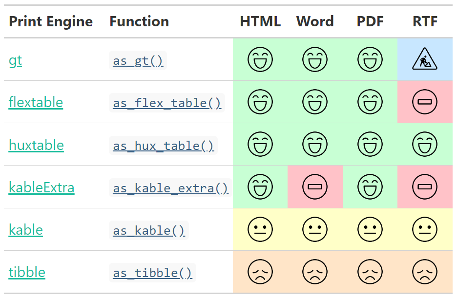
For this manuscript, exporting to a Word document is the most convenient. The easiest way in R to go from table to Microsoft Word is through a flextable object.

  (previous code) %>% as_flex_table()

Flextable output:

You can see that the formatting conversion is less than perfect. It is not trivial to convert formmating stuctures between packages, so I applaud the fact we are more half-way there. At this point, if you export to Word the errors will be carried through - so let’s make our changes using the flextable package and then export to Word.

If you haven’t used Flextable (https://github.com/davidgohel/flextable), I’d put it in the top 5-10 packages to learn if you are using R for academic workflows. Flextable is the easiest route to Microsoft Office and for most of us our editing and collaboration is done through Word documents.

First, let’s go back to our main demographic table code and assign it to a variable so we can play with the formatting.

ft.demographics <- df.demographics %>%
  tbl_summary(include = c(group, sex, visitage),
              by = group,
              type = all_continuous() ~ "continuous2",
              statistic = all_continuous() ~ c("{N_nonmiss}",
                                               "{mean}\u00B1{sd}", 
                                               "{min}, {max}"),
              label = c(sex ~ "Sex", visitage = "Age (years)")) %>% 
  add_p() %>% 
  modify_header(label = "**Measure**") %>% 
  modify_caption("**Table 1. Patient Characteristics**") %>% 
  bold_labels()  %>% 
  modify_spanning_header(all_stat_cols()~ "**Group**") %>% 
  as_flex_table()

I often prefix my variables by the object they contain. In this example, ‘ft’ refers to flextable.

Let’s look at the differences in betwen the table:

1. Numerical values: No difference
2. Column and Row Organization: No difference
3. Title: bold is replaced with markdown ‘**’
4. Legend: Looks ok
5. Headings: not bolded

flextable is easy to work with and so I will refer to the documentation (https://ardata-fr.github.io/flextable-book/) on how to apply bold to the headings.

ft.demographics %>%
  autofit() %>%
  style(part = "header",
    i = 1:2,
    pr_t = fp_text_default(
      bold = TRUE)
  )

The way to read this flextable code is as follows: change the style of rows (i) 1 through 2 1:2 of the header by formatting the text (pr_t) as bold.

Output:

The caption in flextable is a strange entity and doesn’t easily play along with the other formatting options used with rows and tables. Though there is probably a way to style that caption, I am ok doing the final edits in Word (as I will assign them a style).

Finally, let’s export our table to Word using the flextable pipe function save_as_docx and look at our final results:

ft.demographics %>%
  autofit() %>%
  style(part = "header",
    i = 1:2,
    pr_t = fp_text_default(
      bold = TRUE)
  ) %>% save_as_docx(path="srcchirp_table1_demographics.docx")

I am extremely impressed with the final output- my hats off to Daniel Sjoberg and his team. As I have spent countless hours devising scripts to create a similar table, to see it done so quickly really feels like an advancement of our current tools.

Here is the full code to this tutorial: https://www.dropbox.com/s/k72cb5527aj4e6w/srcchirp_results1.R?dl=0

Stick around for Part 2 as we look at making similar tables with response variables.